Support Vector Machines (SVM) Explained

Mastering the art of finding the optimal boundary between classes.

Support Vector Machines (SVM): Finding the Best Divider

Imagine you have a scatter plot with two different groups of dots (say, blue and green). How would you draw a line to separate them? You could draw many possible lines! But which one is the *best*? Support Vector Machine (SVM) is a powerful machine learning algorithm that tackles exactly this problem, aiming to find the optimal boundary between classes.

SVM is primarily used for Classification tasks (though it can be adapted for Regression), and it's known for its effectiveness, especially in high-dimensional spaces (when you have many input features) and situations where the separation isn't perfectly clean.

Main Technical Concept: SVM is a supervised learning algorithm that finds an optimal hyperplane (a decision boundary) that best separates data points belonging to different classes by maximizing the margin (distance) between the hyperplane and the nearest data points of any class (the support vectors).

The Core Idea: Widest Street Possible

Think of the data points for each class as houses in different neighborhoods. SVM tries to draw the widest possible street between the neighborhoods, ensuring the street doesn't touch any houses.

Hyperplane: This is the line (in 2D), plane (in 3D), or hyperplane (in higher dimensions) that acts as the decision boundary – the middle of the street.
Margin: This is the width of the street itself – the empty space between the hyperplane and the nearest houses from *both* neighborhoods. SVM aims to make this margin as wide as possible.
Support Vectors: These are the crucial data points (the "houses") that are closest to the street (the hyperplane/margin). They are the points that actually *define* where the street is drawn. If you moved any other point further away, the street wouldn't change. But if you move a support vector, the optimal street might shift!

Image Credit: Zack Weinberg, based on work by Cushner - Wikimedia Commons, CC BY-SA 3.0

By maximizing the margin, SVM creates a decision boundary that is generally more robust and less sensitive to small variations in the data compared to a boundary that just barely separates the classes.

Handling Real-World Data: From Ideal to Practical

The "widest street" idea works perfectly if the neighborhoods are clearly separated with empty space between them (linearly separable data). But real data is often messy. SVM evolved to handle this:

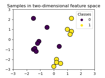
1. Maximal Margin Classifier (The Ideal Case)

This is the original concept: Find the hyperplane with the absolute maximum margin for data that *is* perfectly linearly separable.
Limitation: Extremely sensitive. If even one data point crosses the margin or a new point falls close to it, the optimal hyperplane can change dramatically. It doesn't work if data isn't separable.

2. Support Vector Classifier (SVC) - The Soft Margin

This is a more practical approach that allows for some flexibility. It introduces the idea of a "soft margin".
It allows some data points to be *inside* the margin or even on the *wrong side* of the hyperplane (misclassified).
Why allow errors? To achieve a better overall fit and improve generalization to new data, especially when the data isn't perfectly separable or contains outliers.
This introduces a crucial trade-off: We want to maximize the margin width BUT ALSO minimize the number/severity of margin violations (misclassifications).
This trade-off is controlled by the C parameter (more on this later!).

3. Support Vector Machine (SVM) - Handling Non-Linearity with Kernels

What if the best boundary isn't a straight line at all, but a curve? SVC can only create linear boundaries.
This is where the full power of SVM comes in, using the "Kernel Trick".
The Idea: Kernels are functions that mathematically transform the original input features into a higher-dimensional space. The magic is that data which is not linearly separable in the original space might *become* linearly separable in this higher-dimensional space!
SVM then finds the optimal *linear* hyperplane in this *higher-dimensional* space. When projected back down to the original space, this linear boundary appears as a complex, non-linear boundary.
Common Kernel Functions:
- Linear Kernel: No transformation (equivalent to SVC). Use if data is likely linearly separable.
- Polynomial Kernel: Creates polynomial combinations of features (allowing curved boundaries like parabolas, etc.).
- Radial Basis Function (RBF) Kernel (Gaussian Kernel): A very popular and powerful kernel. It maps data into an infinite-dimensional space, capable of creating very complex, localized boundaries. Often a good default choice to try.
- Sigmoid Kernel: Behaves somewhat similarly to the activation function in neural networks.

Diagram comparing different SVM kernel boundaries (linear, RBF, polynomial) on the same dataset

Image Credit: Scikit-learn Documentation

Tuning Your SVM: Key Parameters C and Gamma

When using SVM (especially SVC with kernels), two hyperparameters are crucial for performance:

1. C (Regularization Parameter)

What it Controls: The trade-off between having a wide margin and minimizing misclassification errors on the training data. It applies to soft margin classifiers (SVC and SVM with non-linear kernels).
Low C value: Prioritizes a wider margin, even if it means misclassifying more training points. Leads to a simpler decision boundary, higher bias, lower variance (less likely to overfit, might underfit). Acts like stronger regularization.
High C value: Prioritizes correctly classifying training points, even if it means a narrower margin. Allows the model to be more complex to fit the data precisely. Leads to lower bias, higher variance (more risk of overfitting). Acts like weaker regularization.
Finding the right C:** Usually done through cross-validation.

2. Gamma (γ) (for RBF, Polynomial, Sigmoid Kernels)

What it Controls: The influence of a single training example. It defines how far the influence of a single point reaches.

Low Gamma value: A point has far-reaching influence. The decision boundary will be smoother and more general. Low gamma means higher bias, lower variance.

High Gamma value: A point has very local influence (only affects points very close to it). The decision boundary can become highly irregular and "wiggly," closely following individual data points, potentially leading to overfitting. High gamma means lower bias, higher variance.

Finding the right Gamma:** Also typically tuned using cross-validation.

Choosing appropriate `C` and `gamma` values is essential for getting good SVM performance.

Implementing SVM in Python (Conceptual)

Scikit-learn provides excellent SVM implementations (`SVC` for classification, `SVR` for regression).

Import `SVC`:** `from sklearn.svm import SVC`

Prepare Data:** Load, preprocess (handle missing values), split into train/test sets.

Feature Scaling:** Crucial! Use `StandardScaler` on X_train and X_test.

Instantiate `SVC`:** `model = SVC(kernel='rbf', C=1.0, gamma='scale', random_state=42)`

Choose your `kernel` ('linear', 'poly', 'rbf', 'sigmoid').

Set `C` (regularization strength).

Set `gamma` (kernel coefficient, often 'scale' or 'auto' are good defaults, or specify a number).

Train:** `model.fit(X_train_scaled, y_train)`

Predict:** `y_pred = model.predict(X_test_scaled)`

Evaluate:** Use Confusion Matrix, Accuracy, Precision, Recall, F1-Score.

(Detailed code examples are available in many tutorials, the focus here is the theory.)

Advantages and Disadvantages of SVM

👍 Pros:

Effective in High-Dimensional Spaces: Works well even when you have many input features (sometimes more features than samples).

Memory Efficient: Uses only a subset of training points (the support vectors) in the decision function.

Versatile Kernels: The kernel trick allows it to model complex, non-linear decision boundaries effectively.

Robust to Overfitting (with proper C/gamma): The margin maximization objective inherently provides some regularization.

👎 Cons:

Computationally Intensive Training: Can be slow to train on very large datasets.

Sensitive to Hyperparameters: Performance heavily depends on choosing the right kernel and tuning the `C` and `gamma` parameters, often requiring careful cross-validation.

Less Interpretable: The decision boundary, especially with kernels like RBF, can be hard to interpret directly compared to, say, decision trees or linear regression coefficients.

Doesn't Directly Provide Probabilities: Basic SVM outputs a class label. Getting well-calibrated probability estimates requires extra steps (though scikit-learn's `SVC` has a `probability=True` option, it's computationally expensive).

SVM Theory: Key Takeaways

SVM is a powerful supervised learning algorithm, primarily used for classification.

It works by finding an optimal hyperplane that separates classes with the maximum margin.

Support Vectors are the data points closest to the margin that define the hyperplane's position.

Soft Margins (controlled by parameter C) allow for some misclassification, making the model more robust to noisy or non-separable data.

The Kernel Trick (using kernels like Linear, Polynomial, RBF) allows SVM to effectively create non-linear decision boundaries by implicitly mapping data to higher dimensions.

Parameter Gamma (γ) controls the influence of individual points in non-linear kernels.

Choosing the right kernel and tuning C and gamma are crucial for good performance.

Test Your Knowledge & Interview Prep

Interview Question

Question 1: What is a "support vector" in the context of SVM, and why are these points important?

Show Answer

Support vectors are the data points from the training set that lie closest to the decision boundary (hyperplane) or within the margin (or even on the wrong side in a soft-margin SVM). They are important because they are the only points that determine the position and orientation of the optimal hyperplane and the margin. Points further away don't influence the boundary.

Question 2: How does the regularization parameter 'C' affect the SVM's decision boundary and its tendency to overfit or underfit?

Show Answer

The 'C' parameter controls the trade-off between maximizing the margin and minimizing classification errors on the training set.
- A low C allows a wider margin and more misclassifications (more tolerance for errors), leading to a simpler model, potentially higher bias, and lower variance (less overfitting, risk of underfitting).
- A high C enforces stricter classification of training points, leading to a narrower margin and fewer misclassifications, potentially resulting in a more complex model, lower bias, and higher variance (risk of overfitting).

Interview Question

Question 3: What is the purpose of using kernels (like RBF or Polynomial) in SVM?

Show Answer

Kernels are used to handle non-linearly separable data. They mathematically transform the original input features into a higher-dimensional space where the data might become linearly separable. SVM then finds a linear hyperplane in this higher-dimensional space. This "kernel trick" allows SVM to create complex, non-linear decision boundaries in the original feature space without explicitly calculating the coordinates in the high-dimensional space, making it computationally efficient.

Question 4: What does the 'gamma' parameter control when using an RBF kernel in SVM?

Show Answer

The 'gamma' parameter defines how much influence a single training example has. A low gamma means a point has far-reaching influence (like a large radius), resulting in a smoother, more general decision boundary. A high gamma means a point has very local influence (like a small radius), leading to a more complex, potentially "wiggly" decision boundary that closely fits the training data, increasing the risk of overfitting.

Interview Question

Question 5: What is the difference between a Maximal Margin Classifier and a Support Vector Classifier (Soft Margin SVM)?

Show Answer

A Maximal Margin Classifier aims to find the hyperplane with the absolute widest margin *only* if the data is perfectly linearly separable. It does not tolerate any points within the margin or misclassified.
A Support Vector Classifier (Soft Margin SVM) is more flexible. It still tries to maximize the margin but allows some data points to violate the margin (be inside it or on the wrong side) to achieve better generalization, especially when data is not perfectly separable or contains outliers. The trade-off is controlled by the C parameter.

Question 6: Why is choosing the right kernel and tuning parameters like C and gamma important for SVM performance?

Show Answer

The choice of kernel determines the type of decision boundary the SVM can create (linear, polynomial, complex RBF). Using the wrong kernel for the data's structure will lead to poor performance. Similarly, the C and gamma parameters control the bias-variance trade-off. Incorrect values can easily lead to significant underfitting (too simple boundary, high bias) or overfitting (too complex boundary fitting noise, high variance). Proper tuning using techniques like cross-validation is essential to find the combination that generalizes best to unseen data.

Interview Question

Question 7: What is a potential drawback of using a very high value for the 'C' parameter in SVM?

Show Answer

A potential drawback of using a very high 'C' value is increased risk of overfitting. A high C forces the model to classify training points correctly, leading to a narrower margin and a more complex decision boundary that might be fitting noise in the training data. This can result in poor performance on new, unseen data.

Support Vector Machines (SVM) Explained

Support Vector Machines (SVM): Finding the Best Divider

The Core Idea: Widest Street Possible

Handling Real-World Data: From Ideal to Practical

1. Maximal Margin Classifier (The Ideal Case)

2. Support Vector Classifier (SVC) - The Soft Margin

3. Support Vector Machine (SVM) - Handling Non-Linearity with Kernels

Tuning Your SVM: Key Parameters C and Gamma

1. C (Regularization Parameter)

2. Gamma (γ) (for RBF, Polynomial, Sigmoid Kernels)

Implementing SVM in Python (Conceptual)

Advantages and Disadvantages of SVM

👍 Pros:

👎 Cons:

SVM Theory: Key Takeaways

Test Your Knowledge & Interview Prep

You may also be interested in