Gaussian Naive Bayes Explained (Part 2: Continuous Data)

The Key Idea: Assuming the Bell Curve

The core idea behind GNB is simple but powerful:

For a given class (e.g., Class 'Yes'), it assumes that the continuous values of a specific feature (e.g., 'Age') are distributed according to a Gaussian (Normal) distribution. It makes the same assumption for Class 'No', but potentially with a different mean and standard deviation.

Why the Gaussian Distribution?

• It's a very common distribution found in nature and many real-world datasets.
• It's mathematically well-understood and defined by just two parameters:
  • Mean (μ): The center of the bell curve.
  • Variance (σ²) or Standard Deviation (σ): How spread out the curve is.

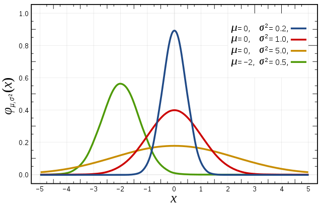
Image Credit: Inductiveload on Wikimedia Commons, CC BY-SA 3.0

Calculating Likelihoods (P(feature | Class))

Instead of counting frequencies, GNB calculates the likelihood using the Gaussian Probability Density Function (PDF). Here's the idea:

1. Calculate Class-Specific Stats: For each class (e.g., 'Yes' and 'No') and for each continuous feature (e.g., 'Age'), calculate the mean (μ) and variance (σ²) of that feature's values *only for the data points belonging to that class*.
2. Use the Gaussian PDF: When you get a new data point with a specific feature value (x), plug this value, along with the calculated mean (μ) and variance (σ²) *for a given class*, into the Gaussian PDF formula to get the likelihood density P(x | Class).

The algorithm calculates this likelihood density for every feature and every class.

Implementing GNB in Python (Scikit-learn)

Scikit-learn makes using Gaussian Naive Bayes very easy with the `GaussianNB` classifier.

Workflow using `Social_Network_Ads.csv`

Let's predict whether a user purchased a product based on 'Age' and 'EstimatedSalary'.

# 1. Import libraries
import numpy as np
import pandas as pd
import matplotlib.pyplot as plt
import seaborn as sns
from sklearn.model_selection import train_test_split
from sklearn.preprocessing import StandardScaler
from sklearn.naive_bayes import GaussianNB
from sklearn.metrics import confusion_matrix, accuracy_score, classification_report

# 2. Load the dataset
dataset = pd.read_csv('Social_Network_Ads.csv')
# Select 'Age' and 'EstimatedSalary' as features, 'Purchased' as target
X = dataset.iloc[:, [2, 3]].values
y = dataset.iloc[:, 4].values

# 3. Split data into Training and Test sets
X_train, X_test, y_train, y_test = train_test_split(X, y, test_size=0.25, random_state=0)

# 4. Feature Scaling (Important for visualization and sometimes GNB)
scaler = StandardScaler()
X_train_scaled = scaler.fit_transform(X_train)
X_test_scaled = scaler.transform(X_test)

# 5. Fit Gaussian Naive Bayes model to the Training set
classifier = GaussianNB()
classifier.fit(X_train_scaled, y_train) # Learns mean & variance per feature per class

# 6. Predict Test set results
y_pred = classifier.predict(X_test_scaled)

# 7. Evaluate the results
# Confusion Matrix
cm = confusion_matrix(y_test, y_pred)
print('Confusion Matrix:\n', cm)

# Accuracy Score
acc = accuracy_score(y_test, y_pred)
print(f'\nAccuracy: {acc:.4f}')

# Classification Report (Precision, Recall, F1-Score)
report = classification_report(y_test, y_pred)
print('\nClassification Report:\n', report)

# 8. Visualize Confusion Matrix (Optional)
plt.figure(figsize=(6, 4))
sns.heatmap(cm, annot=True, fmt='d', cmap='Blues')
plt.title('Confusion Matrix - Gaussian Naive Bayes')
plt.xlabel('Predicted Label')
plt.ylabel('True Label')
# plt.show()
                                    

The code trains the GNB model, makes predictions, and then shows the confusion matrix and other metrics to evaluate how well it performed on the unseen test data.

Common Issues & Considerations

Gaussian Naive Bayes: Key Takeaways

• Gaussian Naive Bayes (GNB) is a type of Naive Bayes classifier specifically designed for continuous numerical features.
• It assumes that features within each class follow a Gaussian (Normal) distribution.
• It calculates the likelihood P(feature | Class) using the Gaussian PDF formula, based on the mean and variance of the feature for that class learned from training data.
• It still relies on the "naive" assumption that features are conditionally independent given the class.
• Requires calculating mean and variance for each feature per class during "training".
• Feature scaling is often recommended for numerical stability and better visualization, although GNB handles scales mathematically.
• It's implemented easily in Scikit-learn using GaussianNB.